Break Even Analysis

Break-Even analysis establishes the relationship among the factors affecting profit. Break-even point usually refers to the number of quantity for which a business neither makes a profit nor incurs a loss.

Fixed Cost

The cost which does not change with change in the volume of production. e.g. taxes, rent etc.

Variable Cost

These cost vary directly with output volume. It is assumed that the ratio between change in cost and change in the level of output remains constant.

Assumptions in Break Even Analysis:

• Selling price (S) will remain constant.
• Linear relationship between sales volume and cost.
• Production and sales quantity (Q) are equal.
•  No other factor, except quantity, will affect the cost.

Break Even Analysis

Let F : Fixed cost, V: variable cost per unit and if Q* is break-even quantity then

F + VQ*  = SQ*

\[Q* = \frac{F}{S-V}\]

Break- Even Point (BEP)

Angle of Incidence (θ)

This is the angle between the lines of total cost and total revenue. Higher is the angle of incidence faster will be the attainment of considerable profit for a given increase in production over BEP. Thus the higher value of θ makes the system more sensitive to changes near BEP.

                      

Profit Volume Ratio:

\[ \frac{S - V}{S}\]

Note: Higher is the profit volume ratio, greater will be the angle of incidence and vice-versa.

(S-V) is contribution margin/gross margin.

Profit Volume graph

Related Topics:

1. Forecasting

2. Queuing Models/Theory

3. PERT And CPM

PERT And CPM

PERT and CPM techniques are used for planning and scheduling large projects.

PERT :  Program Evaluation and Review Technique.
CPM: Critical Path Method.

Terminology:

Network: It consist of series of activities arranged in a logical sequence and shows inter relationship between them.

Activity: It is time consuming effort which is required to perform part of work. It is represented by an arrow ($\to$).

Event: It is the start or completion point of an activity. It is represented by a circle.

Predecessor and Successor Activities: Activities that must be completed before another activity can be started called its predecessor activities. Successor activity occurs following predecessor activities.

Dummy Activity: An activity that consumes no time but shows precedence or relationship among activities. It is represented by dotted line in network.

Each event has two important times associated with it:

Earliest Time: Time when an event can occur when all predecessor activities finished at the earliest possible time.

Latest Time: It is the latest time when each activity can start without delaying the total project.

Forward Pass Computation/ Earliest Start Time

Earliest Start Time (EST): It is the earliest start time of an activity when all predecessor activities are started at their earliest time. 

Earliest Finish Time (EFT): if activity time is 't' then EFT = EST + t

Backward Pass Computation / Latest Time

Latest Finish Time (LFT): The latest finish time for an activity without delaying the project.

Latest Start Time (LST)  = LFT - t

Example:

Example 

Forward Pass:

Starts from initial event to move to end event.

$EST_1$ = 0

$EST_2$ = $EST_1$ + t = 0 + 12 = 12

$EST_3$ = $EST_2$ + 8 = 20

$EST_4$ = $EST_2$ + 10 = 22

$EST_5$ = max{ ($EST_3$+14) , ($EST_4$ + 8) } = max{34, 30} = 34

$EST_6$ = $EST_5$ + 4  = 38

Backward Pass:

Starts from end event to come to first event.

$LST_6$ = 38

$LST_5$ = $LST_6$ - 4 = 34

$LST_4$ = $LST_5$ - 8 = 26

$LST_3$ = $LST_5$ - 14 = 20

$LST_2$ = min{ ($LST_3$ - 8), ($LST_4$ - 10)} = min{12, 16} = 12

$LST_1$ = $LST_2$ - 12 = 0

Slack: Difference between the latest time and earliest time of an event is called slack. An activity with zero slack is known as critical activity.

Critical Path : Critical path is the on the network of project activities which takes longest time from start to finish.
1-2-3-5-6

Total Float: It is the time which completion of an activity can be delayed beyond earliest expected completion time without affecting total project time. 

Total float = Latest start time - Earliest start time

Free Float: It is the time which the completion an activity can be delayed without delaying the earliest start of any succeeding activity.

Free Float = Total Float - Head Event Slack

Independent Float: It is the time which the start of an activity can be delayed without affecting the earliest start time of any immediately following activities assuming that the preceding activity has finished its LFT.

Independent Float = Free Float - Tail Event Slack

PERT :  Program Evaluation and Review Technique

It is used when activity times are not known with certainty. 

The fundamental assumption in PERT is that the three estimates of time ($t_m, t_o, t_p) follow β - distribution curve.

Optimistic Time ($t_o$): It is an estimate of minimum possible time to complete the activity under ideal condition. 

Most Likely time ($t_m$): This lies between optimistic and pessimistic time estimates.

Pessimistic Time ($t_p$): It is the longest time taking into consideration odds.

 Expected time (mean) :

\[t_e = \frac{t_o + 4t_m + t_p}{6}\]

Standard deviation        \( σ = \frac{t_p - t_o}{6}\)

Variance                        \( σ^2 = (\frac{t_p - t_o}{6})^2\)

• Expected time of project ($T_{e}$) is the sum of the expected time of all activities lies on critical path.
• Expected time of activity is assumed to be β - distribution and  expected time for project is normally distributed.
• Variance of the expected time of project ($σ_{cp}^2$) is the sum of the variance of the expected time of all activities along the critical path.
• Probability that the project will be completed  in a given time (T)

Normal distribution $ Z = \frac{T - T_e}{ σ_{cp}}$

Probability P = φ(Z).

For a normal deviate of Z = +1, the corresponding probability is 84.1% , for Z = –1 corresponding P = 15.9 % and for Z = 0 corresponding P = 50%.

Difference Between CPM and PERT:

CPM	PERT
It is activity oriented	It is event oriented
Activity time is deterministic	Activity time is probabilistic
One time estimate	Three time estimates

Queuing Models

The main objective of Queuing model is achievement of an economical balance between the cost of providing service and the cost associated with the waiting time. This theory is used in service oriented organizations like machine repair shop, production shop, restaurant , railway ticket windows banks etc.

Graph of Optimization of cost

Characteristics of Queuing Model

• System : The place where the customer arrives in order to get service is called system.

• Arrival Rate or Arrival Pattern: The average number of customers arriving per unit time within the system to get service is called arrival rate. Arrival is random and if we assume that the arrival is governed by Poisson's distribution then the time between arrivals is exponentially distributed.

          For a given arrival rate (λ) , 

               \[ P(x) = \frac{e^{-λ} λ^x}{x!}\]     

For x = 0,1,2,3,......

P(x) : Probability of x arrival

x: Number of arrival per unit time

The corresponding exponential distribution for inter arrival time is given by

\[P(t) = λ e^{-λt}\]

• Service Rate or Service Pattern : The number of customers serviced per unit time is called service rate. There is no standard probability distribution for service pattern but it is assumed to follow exponential distribution for simplicity.

• Service Rule or Service Discipline: It is about how customers are picked from queue for service. Examples: First Come First Serve (FCFS), Last in first Out(LIFO), Service in Random Order (SIRO) etc.

• Calling Population: The entire sample of customers from which a few visit the service facility is known as calling population. It is assumed finite if arrival rate depends on the number of  customers being served or waiting and assumed if arrival rate is independent of number of  customers being served or waiting. 

Customers Behavior

• Jockey: When customer switches the queue in hope to get service faster.
• Reneging: Customer leaves the system without getting service.
• Balking: If queue is very long, customer decides not to join the queue.
• Cheater: Customer takes illegal means like bribing in hope to to get service faster.

Representation of Queuing Model

Queuing models are represented by Kendall Lee Notaion:

(a/b/c) : (d/e/f)

where, a= probability distribution for arrival pattern              

 b= probability distribution for service pattern 

c = number of servers                                       

d= service rule or service discipline                 

e= size of system                                              

f= size calling population                                 

                  

Single Server Queuing Model (M/M/1) : (FIFO/∞/∞)

λ = Arrival rate (Poisson Distribution)

\( \frac{1}{λ}\) = Inter arrival rate (Exponential) or time gap between two consecutive arrivals

μ = Service rate (exponential) 

If λ > μ then queue length will keep on increasing and at last system will fail.

If λ < μ then System works:

Traffic Intensity(ρ)

The ratio of arrival rate to service rate is called traffic intensity. It is also known as utilization factor or channel efficiency and clearing ratio. 

    \[ ρ = \frac{λ}{μ}\] 

It tells the percentage time server is busy and probability that a customer has to wait.

Some Important formulas

1. Probability that the service facility is idle or probability of zero customers in the system

\[ P_o = 1 - ρ\]

2. Probability of 'n' customers in the system

\[ P_n = ρ^n . P_o\]

\[P_o  + P_1 + P_2 + P_3 + .......... = 1\]

3. Average number of customers in the system: It includes both the customers waiting in the queue and customers which are provided service.

\[ L_s = \sum_{n=0}^{\infty} n. P_n\]

   \[ L_s = \frac{ρ}{1 - ρ}\] 

4. Average number of customers in the queue: It doesn't include the customers which are provided service.

   \[ L_q = \frac{ρ^2}{1 - ρ}\]

5. Average length of non-empty queue or at least one customer in the queue

   \[ L_n = \frac{1}{1 - ρ}\]

Little's Law

It states that average number of customers in the queue or system is equal to average customers arrival rate multiplied by average waiting time in the queue or system respectively. 

\[L_q = λ.W_q   ,  L_s = λ.W_s\]

6. Waiting time of the customer in system

\[ W_s = \frac{L_s}{λ} = \frac{1}{μ - λ}\]

7. Waiting time time of the customer in queue

\[ W_q = \frac{L_q}{λ} = W_s - \frac{1}{μ}\]

7. Probability of 'n' arrivals in time t''

   \[ P(n, t)  = \frac{e^{-λt}{λt}^n}{n!}\]

8. Probability that the waiting time in the queue is greater than or equal to 't'

  \[ P(W_q \geq t)  = \frac{λ}{μ}e^{-(μ - λ)t}\]

9. Probability that the waiting time in the system is greater than or equal to 't'

  \[ P(W_s \geq t)  = e^{-(μ - λ)t}\]

Forecasting

Forecasting is the art of predicting future sales or demand of a product. The survival of any organization depends upon how well they are able to project the demand in future

Types of Demand variation

Time Horizon in Forecasting

1. Short term forecasting               -  1 to 3 months
2. Intermediate term forecasting   -   3 to 12 months
3. Long term forecasting              -    More than a year.

Classification of Forecasting

Types of forecasting

Judgmental Technique

This technique is relies on the art of human judgment i.e. how well a human being can predict the demand of a product in future.

1. Opinion survey
2. Market trial
3. Market research
4. Delphi technique

Time Series Method

In this method, we project the future demand for the product based on the historical pattern of demand.

1) Past Average

In this method forecast is equal to average actual demand of a product for the previous period.

2) Moving Average Method

This method uses past data and calculate a moving average for a constant period. Fresh average is calculated at the end of each period by adding the actual demand data for the most recent period and deleting the data for older period.

Moving average   =  Sum of demands for given period  / chosen number of period

3) Weighted Moving Average

In Moving average method equal weightage is given to demand of each period but this method gives unequal weight to each demand data in such a manner that the summation of all weights always equals to one. More weightage is given to recent demand and least weightage assigned to oldest demand.

Method to find the weightages

if N = Number of periods and have to calculate (N+1)th period forecast;

Sum = N(N+1)/2

Weightage to given recent demand as

N/Sum,  (N-1)/Sum,  (N-2)/Sum, .....   ........  1/Sum

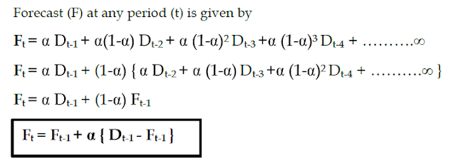
4) Exponential Smoothing Method

When the value of N become very large this method is used. This method assigns weight to all the previous data and the weight assigned are in exponentially decreasing order.

Where,  Ft = Forecast for the period 't'

              Ft-1 = Forecasted demand for the last period 

         

              Dt-1  = Demand for the last period

             

In general, If smoothing constant is not given and is equivalent to

Responsiveness and stability

Responsiveness indicates that the calculated forecast have a fluctuating and swinging pattern where as stability means that the forecast pattern is flat or has less fluctuation. 

Responsiveness is preferred for new product and for that number of period is kept small and stability is preferred for old exiting product and for that number of periods is kept large.

 

Causal Forecasting

It tries to identify the factors which causes the variation of demand and try to establish a relationship between the demand and their factors.

Linear Regression

y = a + bx

yx = ax + bx^2

We get, 

Error Analysis

• Bias

• Bias also called MFE and  it is a measure of over estimation or under estimation.
• A positive Bias means underestimated forecast
• A negative Bias means overestimated forecast

• Mean Square Error(MSE) 

• Mean Absolute Deviation (MAD)

• Mean absolute percentage error (MAPE)

• Tracking Signal(Ts)

Ts tells how well the forecast is predicting the actual value. If value of Ts goes beyond 3*sqrt(MSE) then it indicates that model needs to be revised.